
MATLAB Code for Constellation Diagrams of ASK, FSK, and PSK


MATLAB Script

% The code is developed by SalimWireless.Com

clc;

clear;

close all;


% Parameters

numSymbols = 1000; % Number of symbols to simulate

symbolIndices = randi([0 1], numSymbols, 1); % Random binary symbols (0 or 1)


% ASK Modulation (BASK)

askAmplitude = [0, 1]; % Amplitudes for binary ASK

askSymbols = askAmplitude(symbolIndices + 1); % Modulated BASK symbols


% FSK Modulation (Modified BFSK with 90-degree offset)

fs = 100; % Sampling frequency

symbolDuration = 1; % Symbol duration in seconds

t = linspace(0, symbolDuration, fs*symbolDuration);

fBase = 1; % Base frequency

frequencies = [fBase, fBase]; % Same frequency for both


% Generate FSK symbols with 90° phase offset

fskSymbols = arrayfun(@(idx) ...

    cos(2*pi*frequencies(1)*t) * (1-idx) + ...

    1j * cos(2*pi*frequencies(2)*t) * idx, ...

    symbolIndices, 'UniformOutput', false);


% Extract last points (constellation points)

fskConstellation = cellfun(@(x) x(end), fskSymbols);


% PSK Modulation (BPSK)

pskSymbols = exp(1j * pi * symbolIndices); % Binary PSK symbols in complex plane


% Plotting

figure;


% ASK Constellation Diagram

subplot(1, 3, 1);

scatter(real(askSymbols), zeros(size(askSymbols)), 'filled');

grid on;

title('Binary ASK (BASK) Constellation');

xlabel('In-phase');

ylabel('Quadrature');

axis([-1.5 1.5 -1.5 1.5]);


% FSK Constellation Diagram

subplot(1, 3, 2);

scatter(real(fskConstellation), imag(fskConstellation), 'filled');

grid on;

title('Binary FSK (BFSK) Constellation with 90° Offset');

xlabel('In-phase');

ylabel('Quadrature');

axis([-1.5 1.5 -1.5 1.5]);


% PSK Constellation Diagram

subplot(1, 3, 3);

scatter(real(pskSymbols), imag(pskSymbols), 'filled');

grid on;

title('Binary PSK (BPSK) Constellation');

xlabel('In-phase');

ylabel('Quadrature');

axis([-1.5 1.5 -1.5 1.5]);

web('https://www.salimwireless.com/search?q=ask%20fsk%20psk', '-browser');

Output


Copy the MATLAB Code above from here


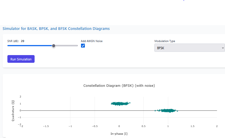
Online Simulators for Constellation Diagrams of ASK, FSK, and PSK


Explore Signal Processing Simulations


Further Reading


Contact Us

Name

Email *

Message *

Popular Posts

LDPC Encoding and Decoding Techniques

Low Density Parity Check (LDPC) Guide Comprehensive analysis of linear error-correcting block codes, Tanner graphs, and 5G-NR implementations. 📘 Overview 🧮 Encoding 🧩 Decoding 📚 Resources Theory Encoding Tech Tanner Graph 5G Encoding Decoding 'LDPC' is the abbreviation for 'low density parity check'. LDPC code H matrix contains very few amount of 1's and mostly zeroes. LDPC codes are error correcting code. Using LDPC codes, channel capacities that are close to the theoretical Shannon limit can be achieved. Low density parity check (LDPC) codes are linear error-correcting block code suitable for error correction in a large block sizes transmi...

Online Simulator for ASK, FSK, and PSK Signal Generation

Interactive Digital Signal Processing (DSP) Tutorial and Simulator for ASK, FSK, and BPSK modulation techniques. Try our new Digital Signal Processing Simulator!   •   Interactive ASK, FSK, and BPSK tools updated for 2025. Start Now Digital Modulation Visualizer: ASK, FSK, & BPSK Simulator Learn and visualize binary modulation techniques (ASK, FSK, BPSK) in real-time with adjustable carrier and sampling parameters. Perfect for DSP students and engineers. 📡 ASK Simulator đŸ“ļ FSK Simulator 🎚️ BPSK Simulator 📚 More Topics ASK Modulator FSK Modulator BPSK Modulator Demodulation More Topics 1. ASK (Ampli...

UGC NET Electronic Science Previous Year Question Papers with Solutions

Download Papers and Solutions Exam Pattern Preparation Tips FAQs More Home / Engineering & Other Exams / UGC NET 2026 PYQ 📊 Exam Highlights: Electronic Science (88) Feature Details Junior Research Fellowship (JRF) ₹37,000 + HRA per month Eligibility M.Sc/M.Tech in Electronics (55%) Validity of Certificate JRF (3 Years) | Lectureship (Lifetime) đŸ“Ĩ Download UGC NET Electronics PDFs Complete collection of previous year question papers, answer keys and explanations for Subject Code 88. Start Downloading 📂 View All Question Papers June 2025 - Question Paper Download PDF June 2025 - Sol...

Gaussian minimum shift keying (GMSK)

📘 Overview & Theory 🧮 Simulator for GMSK 🧮 MSK and GMSK: Understanding the Relationship 🧮 MATLAB Code for GMSK 📚 Simulation Results for GMSK 📚 Q & A and Summary 📚 Further Reading Dive into the fascinating world of GMSK modulation, where continuous phase modulation and spectral efficiency come together for robust communication systems! Core Process of GMSK Modulation Phase Accumulation (Integration of Filtered Signal) After applying Gaussian filtering to the Non-Return-to-Zero (NRZ) signal, we integrate the smoothed signal to produce a continuous phase signal. For GMSK, the modulation index is $h=0.5$, meaning a bit '1' results in a phase shift of $\pi/2$: θ(t) = 2Ī€h ∫ 0 t m filtered (Ī„) dĪ„ This integration is crucial for avoiding abrupt phase transitions, ensuring smooth and continuous phase changes. Phase Mo...

Constellation Diagrams of ASK, PSK, and FSK (with MATLAB Code + Simulator)

Constellation Diagrams: ASK, FSK, and PSK Comprehensive guide to signal space representation, including interactive simulators and MATLAB implementations. 📘 Overview 🧮 Simulator ⚖️ Theory 📈 Q-function 📚 Resources BASK Modulation Transmits one of two signals: 0 or $\sqrt{E_b}$, representing binary 0 and 1. Simple but sensitive to noise. BFSK Modulation Transmits one of two signals: $\sqrt{E_b}$ on the Y-axis or $\sqrt{E_b}$ on the X-axis. These are orthogonal signals. BPSK Modulation Transmits $+\sqrt{E_b}$ or $-\sqrt{E_b}$ (antipodal signaling). Most efficient binary scheme. ...

1G to 5G Technology - Evolution of Wireless Generations

Cellular wireless evolution Generation Frequency band PHY features Data rate Spectral Eff. (bps/Hz) 1G 850 MHz FDMA, FM N/A N/A 2G 900 MHz, 1.8 GHz TDMA/CDMA, GMSK/QPSK, FEC, PC 10 Kbps < 1 3G 1.8–2.5 GHz CDMA, QAM 1–40 Mbps 1–8 4G 2–8 GHz OFDMA, SC-FDMA, QAM, MIMO-OFDM 100–600 Mbps 15 5G 1–6 GHz mm wave (26–28 GHz) < 1 GHz (massive IoT) visible light? massive MIMO, beamforming D2D, Full duplex, NOMA LDPC and Polar codes OFDM & variants (adapted to extremes?) multi-Gbps several tens Waveform design is the major change between the generations Mobile Wireless Generations Specifications  1G  Voice, Analog traffic, FDMA  2G  Voice, SMS, CS data ...

MATLAB Code for OTFS (Orthogonal Time Frequency Space)

MATLAB Code for OTFS (Orthogonal Time Frequency Space) %% Clear workspace clc; clear; close all ; %% Step 1: OTFS Parameters N_delay = 4; % Number of delay bins (rows) N_doppler = 4; % Number of Doppler bins (columns) N_sym = N_delay * N_doppler; modOrder = 4; % QPSK SNR_dB = 20; % Noise level %% Step 2: Generate random data symbols data = randi([0 modOrder-1], N_sym, 1); txSymbols = pskmod(data, modOrder, pi/4); disp( 'Transmitted Delay-Doppler symbols:' ); disp(reshape(txSymbols, N_delay, N_doppler)); %% Step 3: Map Delay-Doppler → Time-Frequency (ISFFT) % ISFFT: Inverse Symplectic Finite Fourier Transform % 1. Take IDFT along Doppler (columns) % 2. Take DFT along Delay (rows) ddSymbols = reshape(txSymbols, N_delay, N_doppler); % Step 3a: IDFT along columns (Doppler) tfGrid = ifft(ddSymbols, N_doppler, 2); %IFFT (accross columns) along Doppler → spreads in time (Delay → Time) %FFT (accross rows)along Delay → spreads in frequency (Delay → Frequency) % Step 3b: DFT along ...