Pulse Amplitude Modulation (PAM) & Demodulation
Pulse Amplitude Modulation (PAM) & Demodulation of an Analog Message Signal
MATLAB Script
clc;
clear all;
close all;
fm = 10; % frequency of the message signal
fc = 100; % frequency of the carrier signal
fs = 1000 * fm; % sampling frequency (100 kHz)
t = 0:1/fs:1;
m = 1 * cos(2 * pi * fm * t);
c = 0.5 * square(2 * pi * fc * t) + 0.5;
s = m .* c;

subplot(4,1,1);
plot(t,m);
title('Message signal');
xlabel('Time');
ylabel('Amplitude');

subplot(4,1,2);
plot(t,c);
title('Carrier signal');
xlabel('Time');
ylabel('Amplitude');

subplot(4,1,3);
plot(t,s);
title('Modulated signal');
xlabel('Time');
ylabel('Amplitude');

% Demodulation
d = s .* c;
filter = fir1(200,fm/fs,'low');
original_t_signal = conv(filter,d);
t1 = 0:1/(length(original_t_signal)-1):1;

subplot(4,1,4);
plot(t1,original_t_signal);
title('Demodulated signal');
xlabel('Time');
ylabel('Amplitude');

web('https://www.salimwireless.com/search?q=pulse%20amplitude%20modulation', '-browser');
Output

Another Code for Pulse Amplitude Modulation and Demodulation of an Analog Message Signal
MATLAB Script
clc;
clear;
close all;

% Parameters
messageFrequency = 2;
carrierFrequency = 20;
samplingFrequency = 1000;
duration = 1;
A = 1;

% Time vector
t = 0:1/samplingFrequency:duration;

% Message signal
messageSignal = A * sin(2 * pi * messageFrequency * t);

% Carrier signal
carrierSignal = A * square(2 * pi * carrierFrequency * t);

% PAM signal
pamSignal = messageSignal .* (carrierSignal > 0);

% Plotting
figure;
subplot(3,1,1); plot(t, messageSignal); title('Message Signal');
subplot(3,1,2); plot(t, carrierSignal); title('Carrier Signal');
subplot(3,1,3); plot(t, pamSignal); title('PAM Signal');

web('https://www.salimwireless.com/search?q=pulse%20amplitude%20modulation', '-browser');
Pulse Amplitude Modulation (PAM) & Demodulation for Digital Data
% The code is written by SalimWireless.Com
clc;
clear;
close all;

% Parameters
M = 8;
numSymbols = 100;
Fs = 1000;
T = 1;

% Generate random data
data = randi([0 M-1], 1, numSymbols);

% PAM Modulation
pamLevels = linspace(-M + 1, M - 1, M);
modulatedSignal = pamLevels(data + 1);

% Create time vector
t = 0:1/Fs:T*numSymbols-1/Fs;

% Upsample and create PAM signal
upsampledSignal = zeros(1, length(t));
for i = 1:numSymbols
    upsampledSignal((i-1)*Fs+1:i*Fs) = modulatedSignal(i);
end

% Add noise
snr = 20;
noisySignal = awgn(upsampledSignal, snr, 'measured');

% PAM Demodulation
receivedSymbols = noisySignal(1:Fs:end);
demodulatedData = zeros(1, numSymbols);
for i = 1:numSymbols
    [~, demodulatedData(i)] = min(abs(receivedSymbols(i) - pamLevels));
end

% Plotting
figure;
subplot(4,1,1); stem(data); title('Original Data');
subplot(4,1,2); plot(t, upsampledSignal); title('Transmitted PAM Signal');
subplot(4,1,3); plot(t, noisySignal); title('Received Noisy PAM Signal');
subplot(4,1,4); stem(demodulatedData); title('Demodulated Data');
grid on;

disp('Original Data:'); disp(data);
disp('Demodulated Data:'); disp(demodulatedData);

web('https://www.salimwireless.com/search?q=pulse%20amplitude%20modulation', '-browser');
Output

| Parameter | PAM | PWM | PPM | DM | PCM |
|---|---|---|---|---|---|
| What is varied? | Amplitude | Width | Position | Delta (difference) | Binary code |
| Pulse Width | Constant | Variable | Constant | Constant | Constant |
| Noise Immunity | Low | Moderate | High | Moderate | High |
| Bandwidth | Low | Medium | High | Low | High |
| Complexity | Simple | Moderate | Complex | Simple | Complex |
| MATLAB Code | PAM Script | PWM Script | PPM Script | DM Script | PCM Script |
| Detailed Study | PAM | PWM | PPM | DM | PCM |
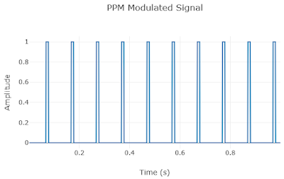
Simulation Results for Comparison of PAM, PWM, PPM, DM, and PCM


Instructions for Pulse Amplitude Modulation (PAM)
- Note: Use the input fields to enter the message frequency and the square pulse carrier frequency.
- Step 1: Click the "Generate Message" button to generate the input message signal.
- Step 2: Click the "Generate Carrier" button to generate the carrier signal. Carrier must be > Message.
- Step 3: Click the "Generate PAM Signal" button to generate the Modulated signal.
PAM Modulation Control Center
Perform Pulse Amplitude Modulation by interacting with the signal generators below.
Ready for Signal Recovery?
After generating your PAM signal, proceed to the Demodulation section to recover the original message using a reconstruction filter.
Go to DemodulationInstructions for Pulse Amplitude Demodulation
- The reconstruction filter recovers the original message from the sampled PAM signal.
- A low-pass filter (LPF) is used with a cutoff frequency at or above the message frequency.
- Click 'Demodulate' to view the recovered baseband signal.
Technical Definition: PAM Signal
MATLAB Mathematical Representation
Copy Snippet
% Ideal Sampling with Pulse Train
t = 0:0.001:1;
fm = 2; fc = 10;
m_t = cos(2*pi*fm*t);
c_t = square(2*pi*fc*t);
s_pam = m_t .* (c_t > 0);
% Low Pass Reconstruction
[b,a] = butter(4, fm/(fs/2));
demod = filter(b,a, s_pam);
Advanced PAM Simulator (Try real signal)
Upload CSV, .wav, or .mp4
Parameters
Actual Sample Rate (fs): -- Hz
By default, the test signal is 5 Hz, and the pusle carrier signal is 50 Hz.
On this page, you can test real signals just as you would in MATLAB. If you want to access basic signal processing simulations, you can visit the page below. In that page, you can generate CSV files for signals such as the message signal, modulated signal, and others. After generating the files, you can return to this page to analyze the signals.
Further Reading
- Pulse Amplitude Modulation and Demodulation theory
- Is PAM a Digital Modulation Technique ?
- Pulse Width Modulation (PWM) and Demodulation
- Pulse Position Modulation (PPM) and Demodulation
- Delta Modulation and demodulation
- Pulse Code Modulation (PCM)
- Quantization Signal to Noise Ration (Q-SNR)
- MATLAB Code for Pulse Width Modulation and Demodulation
- MATLAB Code for Pulse Position Modulation (PPM) and Demodulation
- MATLAB Code for Pulse Code Modulation (PCM) and demodulation